TensorFlow - 삼목 게임 학습

---

개요

 tic-tac-toe.csv의 삼목 게임을 tensorflow로 학습합니다.  전체 959개의 데이터 중 70%를 학습 데이터로, 30%를 테스트 데이터로 사용하며 learning_rate, epoch, 최적화 알고리즘, 손실 함수에 따라 달라지는 결과를 비교하도록 합니다. 손실 함수로는 평균 제곱 오차(MSE), 다중 분류(CCE; Categorical Cross Entropy)를 사용하며, 최적화 알고리즘으로는 RMSprop(), Adam(), SDG(), Adagrad()를 사용합니다.

GitHub - woorinlee/tic-tac-toe-learning: Tic Tac Toe learning using TensorFlow

---

준비 과정

import tensorflow as tf
from tensorflow.keras.optimizers import RMSprop, Adam, SGD, Adagrad
import numpy as np
import pandas as pd
import matplotlib.pyplot as plt

학습 전, 필요한 패키지들을 import합니다.

ttt_data_csv = pd.read_csv("./tic-tac-toe.csv")

ttt_data_csv.replace(to_replace = "o", value = "1", inplace=True)
ttt_data_csv.replace(to_replace = "b", value = "0", inplace=True)
ttt_data_csv.replace(to_replace = "x", value = "-1", inplace=True)

ttt_data_csv.to_csv("tic-tac-toe-conv.csv", index = False)

기존 데이터	o	b	x
대체 데이터	1	0	-1

pandas를 통해 tic-tac-toe.csv의 o, b, x를 각각 1, 0, -1로 대체한 후 저장합니다.

def load_ttt(shuffle = False):
    label = {'True' : 1, 'False' : 0}
    data = np.loadtxt("./tic-tac-toe-conv.csv", skiprows = 1, delimiter = ",",
        converters = {9: lambda name: label[name.decode()]})
    if shuffle:
        np.random.shuffle(data)
    return data

 numpy의 loadtxt 함수를 통해 csv 파일을 열고, 항목 인덱스 9의 문자열을 {'True' : 1, 'False' : 0}의 정수 레이블로 변환합니다. 이후 numpy의 random.shuffle을 통해 매개변수로 True가 입력되면 변환된 내용의 순서를 섞은 후 반환합니다.

def train_test_data_set(ttt_data, test_rate = 0.3):
    n = int(ttt_data.shape[0] * (1 - test_rate))
    x_train = ttt_data[:n, :-1]
    y_train = ttt_data[:n, -1]

    x_test = ttt_data[n:, :-1]
    y_test = ttt_data[n:, -1]

    return (x_train, y_train), (x_test, y_test)

전체 959개의 데이터 중 70%를 학습 데이터로, 30%를 테스트 데이터로 사용하도록 합니다.

def MSE(y, t):
    return tf.reduce_mean(tf.square(y - t))

CCE = tf.keras.losses.CategoricalCrossentropy()

손실 함수 MSE, CCE를 작성합니다.

ttt_data = load_ttt(shuffle = True)
(x_train, y_train), (x_test, y_test) = train_test_data_set(ttt_data, test_rate = 0.3)

print("x_train.shape:", x_train.shape)
print("y_train.shape:", y_train.shape)
print("x_test.shape:",  x_test.shape)
print("y_test.shape:",  y_test.shape)

 load_ttt 함수에 shuffle 값으로 True를 입력한 후 반환된 값을 ttt_data에 저장합니다. 이후 해당 값을 train_test_data_set 함수를 통해 학습 데이터와 테스트 데이터로 변환합니다. 이후 각 데이터의 개수를 출력합니다.

y_train = tf.keras.utils.to_categorical(y_train)
y_test = tf.keras.utils.to_categorical(y_test)

 만약 손실 함수가 MSE 또는 CCE 이라면 tf.keras.utils.to_categorical()을 통해 y_train과 y_test를 One-Hot 인코딩으로 변환하도록 합니다.

n = 10
model = tf.keras.Sequential()
model.add(tf.keras.layers.Dense(units=n, input_dim=9, activation='sigmoid'))
model.add(tf.keras.layers.Dense(units=2, activation='softmax'))
model.summary()

 은닉층의 뉴런 개수를 10개로 하고, 입력 데이터를 9개, 출력 데이터를 2개로 하며 출력층의 활성 함수가 activation=‘softmax’인 신경망을 생성합니다.

---

학습 과정

opt = RMSprop(learning_rate=0.01)
# opt = Adam(learning_rate=0.01)
# opt = SGD(learning_rate=0.01)
# opt = Adagrad(learning_rate=0.01)

최적화 알고리즘을 설정합니다. (RMSprop)

model.compile(optimizer=opt, loss= MSE, metrics=['accuracy'])
# model.compile(optimizer=opt, loss= CCE, metrics=['accuracy'])

손실 함수를 설정합니다. (MSE)

ret = model.fit(x_train, y_train, epochs=100, verbose=0)

print("len(model.layers):", len(model.layers))
loss = ret.history['loss']
accuracy = ret.history['accuracy']

epochs 값을 100으로 설정합니다.

plt.plot(loss)
plt.xlabel('epochs')
plt.ylabel('loss')
plt.show()

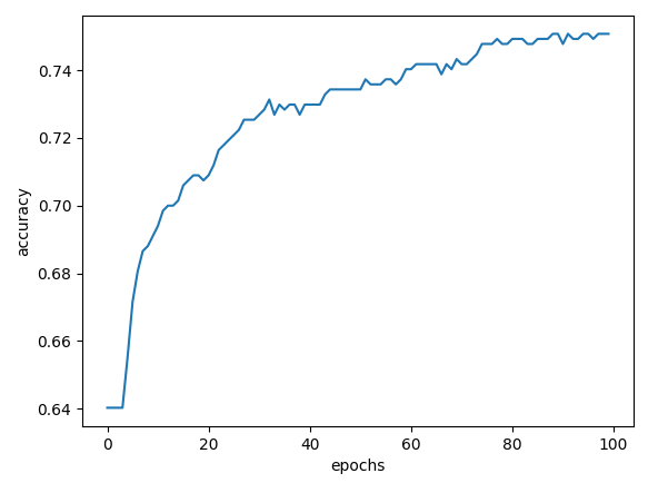
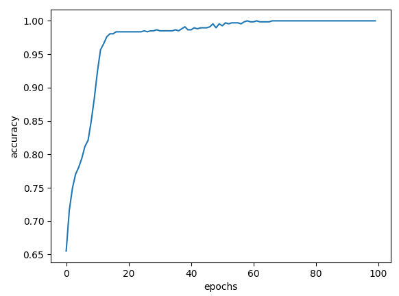
plt.plot(accuracy)
plt.xlabel('epochs')
plt.ylabel('accuracy')
plt.show()

train_loss, train_acc = model.evaluate(x_train, y_train, verbose=2)
test_loss, test_acc = model.evaluate(x_test,  y_test, verbose=2)
y_pred = model.predict(x_train)
y_label = np.argmax(y_pred, axis = 1)
C = tf.math.confusion_matrix(np.argmax(y_train, axis = 1), y_label)
print("confusion_matrix(C):", C)

loss 변화율과 accuracy 변화율을 출력하고 손실율, 정확도를 출력합니다.

---

학습 결과

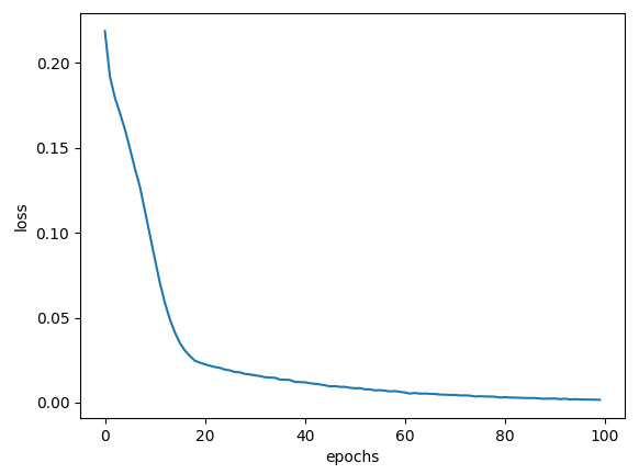
RMSprop, learning_late = 0.01, MSE, epochs = 100에 대한 결과는 다음과 같습니다.

loss 변화율	accuracy 변화율

출력 내용

훈련 데이터 정확도	테스트 데이터 정확도
100%	99.65%

---

학습 결과 비교 분석

1. learning_late

기존 learning_late 값인 0.01보다 큰 0.1 값을 사용하여 결과를 도출한다.

	loss 변화율	accuracy 변화율
learning_late=0.01
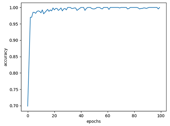
learning_late=0.1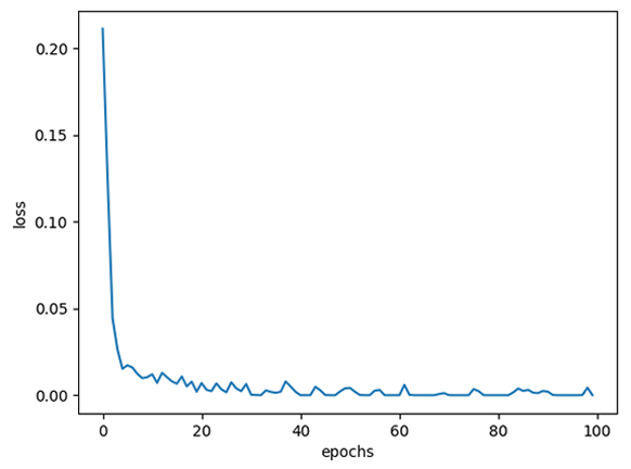

조건	출력 내용
learning_late=0.01
learning_late=0.1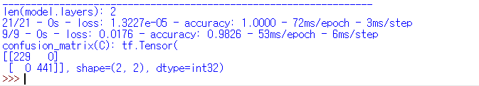

	훈련 데이터 정확도	테스트 데이터 정확도
learning_late=0.01	100%	99.65%
learning_late=0.1	100%	98.26%

 

2. epochs

기존 epochs 값인 100보다 작은 200 값을 사용하여 결과를 도출한다.

	loss 변화율	accuracy 변화율
epochs=100
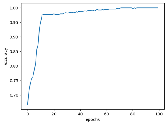epochs=200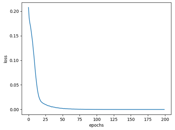

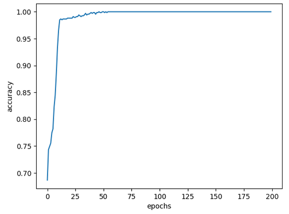조건	출력 내용
epochs=100
epochs=200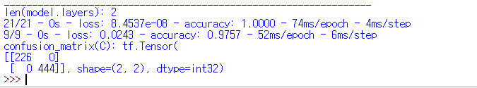

	훈련 데이터 정확도	테스트 데이터 정확도
epochs=100	100%	99.65%
epochs=200	100%	97.57%

 

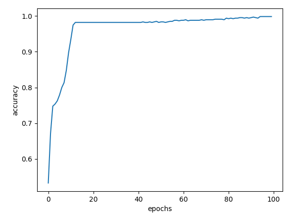
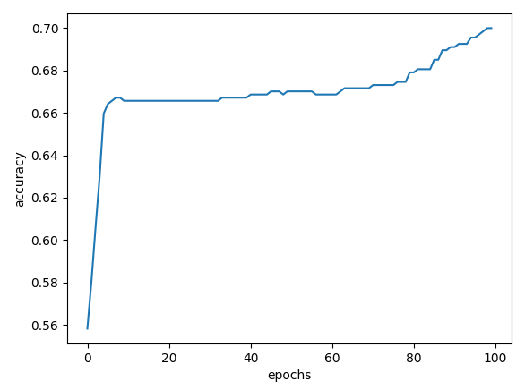
3. 최적화 알고리즘

RMSprop(), Adam(), SDG(), Adagrad() 최적화 알고리즘에 대한 결과를 도출한다.

	loss 변화율	accuracy 변화율
RMSprop()
Adam()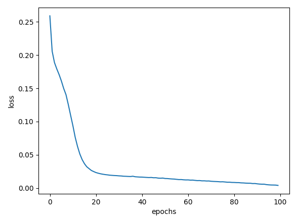
SDG()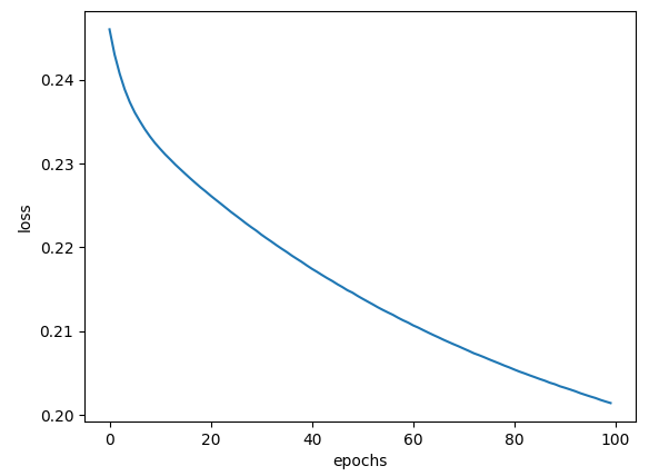
Adagrad()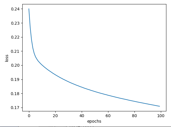

	출력 내용
RMSprop()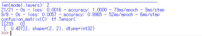
Adam()
SDG()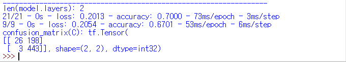
Adagrad()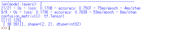

	훈련 데이터 정확도	테스트 데이터 정확도
RMSprop()	100%	99.65%
Adam()	99.85%	98.26%
SDG()	70%	67.01%
Adagrad()	75.07%	76.39%

 

4. 손실 함수

MSE, CCE 손실 함수에 대한 결과를 도출한다.

	loss 변화율	accuracy 변화율
MSE
CCE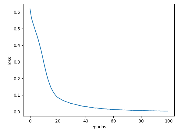

	출력 내용
MSE
CCE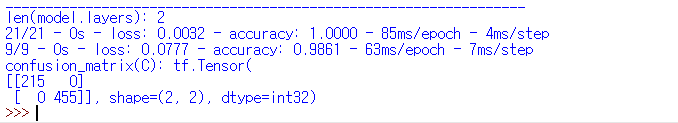

	훈련 데이터 정확도	테스트 데이터 정확도
MSE	100%	99.65%
CCE	100%	98.61%

---

전체 프로그램 코드

import tensorflow as tf
from tensorflow.keras.optimizers import RMSprop, Adam, SGD, Adagrad
import numpy as np
import pandas as pd
import matplotlib.pyplot as plt

# csv 파일 열기
ttt_data_csv = pd.read_csv("./tic-tac-toe.csv")

# o, b, x를 각각 1, 0, -1로 대체 / True, False를 각각 1, 0으로 교체
ttt_data_csv.replace(to_replace = "o", value = "1", inplace=True)
ttt_data_csv.replace(to_replace = "b", value = "0", inplace=True)
ttt_data_csv.replace(to_replace = "x", value = "-1", inplace=True)

# index 속성에 False 값을 주고 "tic-tac-toe-conv.csv" 파일에 저장
ttt_data_csv.to_csv("tic-tac-toe-conv.csv", index = False)

# 수정된 csv 파일 열기
def load_ttt(shuffle = False):
    # 항목 인덱스 9의 문자열을 {'True' : 1, 'False' : 0}의 정수 레이블로 변환
    label = {'True' : 1, 'False' : 0}
    data = np.loadtxt("./tic-tac-toe-conv.csv", skiprows = 1, delimiter = ",",
                      converters = {9: lambda name: label[name.decode()]})
    # shuffle = True이면 순서를 섞은 후 반환
    if shuffle:
        np.random.shuffle(data)
    return data

# 훈련 데이터 70%(670개), 테스트 데이터 30%(288개)로 분리 
def train_test_data_set(ttt_data, test_rate = 0.3):
    n = int(ttt_data.shape[0] * (1 - test_rate))
    x_train = ttt_data[:n, :-1]
    y_train = ttt_data[:n, -1]

    x_test = ttt_data[n:, :-1]
    y_test = ttt_data[n:, -1]

    return (x_train, y_train), (x_test, y_test)

ttt_data = load_ttt(shuffle = True)
(x_train, y_train), (x_test, y_test) = train_test_data_set(ttt_data, test_rate = 0.3)

# 각 데이터 개수 출력 
print("x_train.shape:", x_train.shape)
print("y_train.shape:", y_train.shape)
print("x_test.shape:",  x_test.shape)
print("y_test.shape:",  y_test.shape)

# 손실 함수가 MSE 또는 categorical_crossentropy 이라면
# tf.keras.utils.to_categorical()을 통해 y_train과 y_test를 One-Hot 인코딩으로 변환
y_train = tf.keras.utils.to_categorical(y_train)
y_test = tf.keras.utils.to_categorical(y_test)

# 은닉층의 뉴런 개수 
n = 10
model = tf.keras.Sequential()
# 입력 데이터 9개
model.add(tf.keras.layers.Dense(units=n, input_dim=9, activation='sigmoid'))
# 출력층의 활성 함수가 activation='softmax'인 신경망 생성 / 출력 데이터 2
model.add(tf.keras.layers.Dense(units=2, activation='softmax'))
model.summary()

# MSE 함수 정의
def MSE(y, t):
    return tf.reduce_mean(tf.square(y - t))

# categorical_crossentropy
CCE = tf.keras.losses.CategoricalCrossentropy()

# learning_rate 0.01로 설정 / optimizer RMSprop로 설정  
opt = RMSprop(learning_rate=0.01)
# opt = Adam(learning_rate=0.01)
# opt = SGD(learning_rate=0.01)
# opt = Adagrad(learning_rate=0.01)

# loss
# model.compile(optimizer=opt, loss= MSE, metrics=['accuracy'])
model.compile(optimizer=opt, loss= CCE, metrics=['accuracy'])

# epochs 100으로 설정
ret = model.fit(x_train, y_train, epochs=100, verbose=0)

print("len(model.layers):", len(model.layers))
loss = ret.history['loss']
accuracy = ret.history['accuracy']

# loss 변화율 출력 
plt.plot(loss)
plt.xlabel('epochs')
plt.ylabel('loss')
plt.show()

# accyracy 변화율 출력 
plt.plot(accuracy)
plt.xlabel('epochs')
plt.ylabel('accuracy')
plt.show()

train_loss, train_acc = model.evaluate(x_train, y_train, verbose=2)
test_loss, test_acc = model.evaluate(x_test,  y_test, verbose=2)
y_pred = model.predict(x_train)
y_label = np.argmax(y_pred, axis = 1)
C = tf.math.confusion_matrix(np.argmax(y_train, axis = 1), y_label)
print("confusion_matrix(C):", C)

---

참고 웹사이트

GitHub - datasets/tic-tac-toe: This dataset contains tic-tac-toe endgame snapshots with the information if x player won or lost

tic-tac-toe.csv 데이터 파일 제공

---